Indexing Billions of Text Vectors
Optimizing memory-usage for approximate nearest neighbor search
A frequently occurring problem within information retrieval is the one of finding similar pieces of text. As described in our previous posts (A New Search Engine and Building a Search Engine from Scratch), queries are an important building block at Cliqz. A query in this context can either be a user-generated one, (i.e. the piece of text that a user enters into a search engine), or a synthetic one generated by us. A common use case is that we want to match an input query with other queries already in our index. In this post we will see how we are able to build a system that solves this task at scale using billions of queries without spending a fortune (which we do not have) on server infrastructure.
Let us first formally define the problem:
Given a fixed set of queries , an input query and an integer , find a subset of queries , such that each query is more similar to than every other query in .
For example, with the following set of queries :
{tesla cybertruck, beginner bicycle gear, eggplant dishes, tesla new car, how expensive is cybertruck, vegetarian food, shimano 105 vs ultegra, building a carbon bike, zucchini recipes} |
and , we might expect the following results:
| Input query | Similar queries |
|---|---|
tesla pickup | {tesla cybertruck, tesla new car, how expensive is cybertruck} |
best bike 2019 | {shimano 105 vs ultegra, beginner bicycle gear, building a carbon bike} |
cooking with vegetables | {eggplant dishes, zucchini recipes, vegetarian food} |
Note that we have not yet defined similar. In this context, it can mean almost anything, but it usually boils down to some form of keyword or vector based similarity. With keyword based similarity we can consider two queries similar if they have enough words in common. For example, the queries opening a restaurant in munich and best restaurant of munich are similar because they share the words restaurant and munich, whereas best restaurant of munich and where to eat in munich are less similar because they only share a single word. Someone looking for a restaurant in Munich will however likely be better served by considering the second pair of queries to be similar. This is where vector based matching comes into play.
Embedding Text into Vector Spaces
Word embedding is a machine-learning technique in Natural Language Processing for mapping text or words to vectors. By moving the problem into a vector space we can use mathematical operations, such as summing or computing distances, on the vectors. We can even use conventional vector clustering techniques to link together similar words. It is not necessarily obvious what these operations mean in the original space of words but the benefit is that we now have a rich set of mathematical tools available to us. The interested reader may want to have a look at e.g. word2vec[1] or GloVe[2] for more information about word vectors and their applications.
Once we have a way of generating vectors from words, the next step is to combine them into text vectors (also known as document or sentence vectors). A simple and common way of doing this is to sum (or average) the vectors for all the words in the text together.
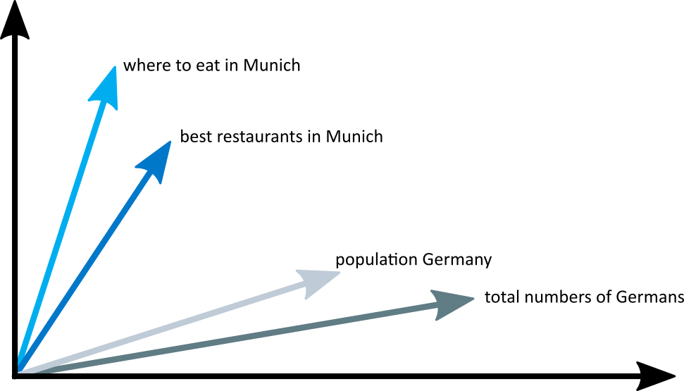
We can decide how similar two snippets of text (or queries) are by mapping them both into a vector space and computing a distance between the vectors. A common choice is to use the angular distance.
All in all, word embedding allows us to do a different kind of text matching that complements the keyword-based matching mentioned above. We are able to explore the semantic similarity between queries (e.g. best restaurant of munich and where to eat in munich) in a way that was not possible before.
Approximate Nearest Neighbor Search
We are now ready to reduce our initial query matching problem into the following:
Given a fixed set of query vectors , an input vector and an integer , find a subset of vectors , such that the angular distance from to each vector is smaller than to every other vector in .
This is called the nearest neighbor problem and plenty of algorithms[3] exist that can solve it quickly for low dimensional spaces. With word embeddings on the other hand, we are normally working with high-dimensional vectors (100-1000 dimensions). In this case, exact methods break down.
There is no feasible way of quickly obtaining the nearest neighbors in high-dimensionsional spaces. In order to overcome this, we will make the problem simpler by allowing for approximate results, i.e. instead of requiring the algorithm to always return exactly the closest vectors, we accept getting only some of the closest neighbors or somewhat close neighbors. We call this the approximate nearest neighbor (ANN) problem and it is an active area of research.
Hierarchical Navigable Small-World Graph
Hierarchical Navigable Small-World graph[4], or HNSW for short, is one of the faster approximate nearest neighbor search algorithms. The search index in HNSW is a multi-layered structure where each layer is a proximity graph. Each node in the graph corresponds to one of our query vectors.
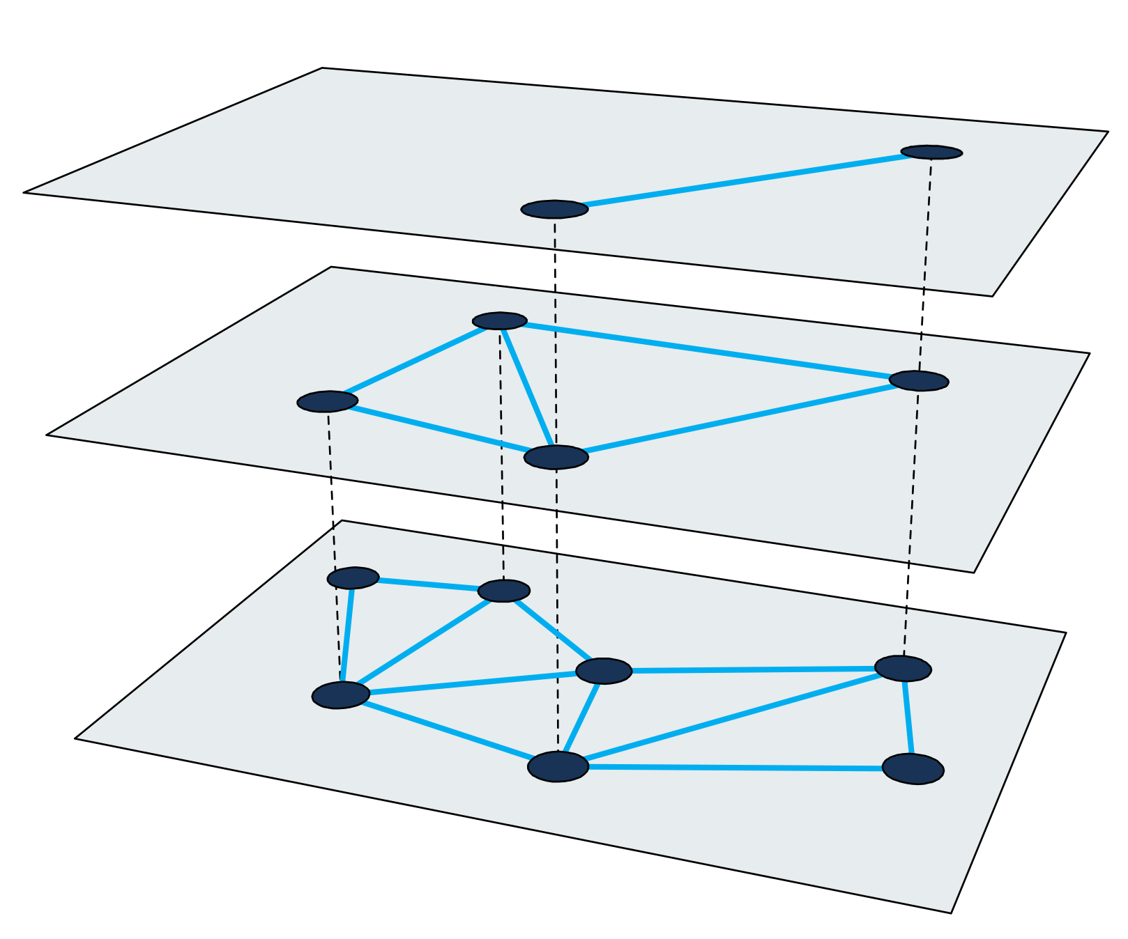
A nearest neighbor search in HNSW uses a zooming-in approach. It starts at an entrypoint node in the uppermost layer and recursively performs a greedy graph traversal in each layer until it reaches a local minimum in the bottommost one.
Details about the inner-workings of the algorithm and how the search index is constructed is well described in the paper[4:1] itself. The important take-away is that each nearest neighbor search consists in performing a graph traversal, where nodes in the graph are visited and distances are computed between vectors. The following sections will outline the steps taken in order to be able to use this method for building a large scale index at Cliqz.
Challenges of Indexing Billions of Queries
Let us assume that the goal is to index 4 billion 200-dimensional query vectors where each dimension is represented by a 4 byte floating-point number[5]. A back-of-the-envelope calculation tells us that the size of the vectors alone is around 3 TB. Since many of the existing ANN libraries are memory-based, this means that we would need a very large server in order to fit just the vectors into RAM. Note that this is the size excluding the additional search index required in most of the methods.
Throughout the history of our search engine, we have had a few different approaches addressing this size problem. Let us revisit a couple of them.
A Subset of the Data
The first and simplest approach, which did not really solve the problem, was to limit the number of vectors in the index. By using only one tenth of all the available data, we could, unsurprisingly, build an index requiring only 10% of the memory as compared to one containing all of data. The drawback of this approach is that search quality suffers, since we have fewer queries to match against.
Quantization
The second approach was to include all data, but to make it smaller through quantization[6][7]. By allowing some rounding errors we can replace each 4 byte float in the original vector with a quantized 1 byte version. This reduces the amount of RAM required for the vectors by 75%. Despite this significant size reduction we need to fit almost 750 GB in RAM (still ignoring the size of the index structure itself), which still requires us to use a very large server.
Tackling Memory Problems with Granne
The approaches above did have merit, but they were lacking in cost efficiency and quality. Even though there are ANN libraries producing reasonable recall in less than 1 ms[8], for our use case we can accept sacrificing some of that speed for reduced server costs.
Granne (graph-based approximate nearest neighbors) is a HNSW-based library developed and used at Cliqz to find similar queries. It is open-source, but still under active development. An improved version is on the way and will be published on crates.io in 2020. It is written in Rust with language bindings for Python and is designed for billions of vectors and with concurrency in mind. More interesting in the context of query vectors, is that Granne has a special mode that uses drastically less memory than previously available libraries.
Compact Representation of Query Vectors
Reducing the size of the query vectors themselves will give the most benefit. In order to do so, we will have to take a step back and consider how the query vectors are created in the first place. Since our queries consist of words and our query vectors are sums of word vectors, we can avoid storing the query vectors explicitly and compute them whenever they are needed.
We could store the queries as a set of words and use a look-up table to find the corresponding word vector. However, we avoid the indirection by storing each query as a list of integer ids corresponding to the vectors of the words in the query. For example, we store the query best restaurant of munich as
where is the id of the word vector for best, and so on. Assuming we have less than 16 million word vectors (more than that comes at a price of 1 byte per word), we can use a 3 byte representation for each word id. Thus, instead of storing 800 bytes (or 200 bytes in the case of the quantized vector) we only need to store 12 bytes[9] for this query.
Regarding the word vectors: we still need them. However, there are a lot fewer words than queries one can create by combining those words. Since they are so few in comparison to the queries, their size does not matter as much. By storing the 4 byte floating-point version of the word vectors in a simple array , we need less than 1 GB per million of them, which can easily be stored in RAM. The query vector from the example above is then obtained as:
The final size of the query representation naturally depends on the combined number of words in all queries, but for 4 billion of our queries the total size ends up being around 80 GB (including the word vectors). In other words, we see a reduction in size by more than 97% compared to the original query vectors or around 90% compared to the quantized vectors.
There is one concern that still needs to be addressed. For a single search, we need to visit around 200-300 nodes in the graph. Each node has 20-30 neighbors. Consequently, we need to compute the distance from the input query vector to 4000-9000 of the vectors in the index and before that, we need to generate the vectors. Is the time penalty for creating the query vectors on the fly too high?
It turns out that, with a reasonably new CPU, it can be done in a few milliseconds. For a query that earlier took a millisecond, we will now need around 5 ms. But at the same time, we are reducing the RAM usage for the vectors by 90%—a trade-off we gladly accept.
Memory Mapping Vectors and Index
So far, we have focused solely on the memory footprint of the vectors. However, after the significant size reduction above, the limiting factor becomes the index structure itself, and we thus need to consider its memory requirements as well.
The graph structure in Granne is compactly stored as adjacency lists with a variable number of neighbors per node. Thus, almost no space is wasted on metadata. The size of the index structure depends a lot on the construction parameters and the properties of the graph. Nevertheless, in order to get some idea about the index size, it suffices to say that we can build a useable index for the 4 billion vectors with a total size of around 240 GB. This might be acceptable to use in-memory on a large server, but we can actually do even better.

An important feature of Granne is its ability to memory map[10] the index and the query vectors. This enables us to lazily load the index and share the memory between processes. The index and query files are actually split into separate memory mapped files and can be used with different configurations of SSD/RAM placement. If latency requirements are a bit less strict, by placing the index file on a SSD and the query file in RAM, we still obtain a reasonable query speed without paying for an excessive amount of RAM. At the end of this post, we will see what this trade-off looks like.
Improving Data Locality
In our current configuration, where the index is placed on a SSD, each search requires up to 200-300 read operations from the SSD. We can try to increase the data locality by ordering elements whose vectors are close so that their HNSW nodes are also closely located in the index. Data locality improves performance because a single read operation (usually fetching 4 kB or more) becomes more likely to contain other nodes needed for the graph traversal. This, in turn, reduces the number of times we need to fetch data during a single search.

It should be noted that reordering the elements does not change the results, but is merely a way of speeding up the search. This means that any ordering is fine, but not all of them will give a speed up. It is likely very difficult to find the optimal ordering. However, a heuristic that we have used sucessfully consists in sorting the queries based on the most important word in each query.
Conclusion
At Cliqz, we are using Granne to build and maintain a multi-billion query vector index for similar query search with relatively low memory requirements. Table 1. summarizes the requirements for the different methods. The absolute numbers for the search latencies should be taken with a grain of salt, since they are highly dependent on what is considered an acceptable recall, but they should at least give a hint about the relative performance between the methods.
| Baseline | Quantization | Granne (RAM only) | Granne (RAM+SSD) | |
|---|---|---|---|---|
| Memory | 3000 + 240 GB | 750 + 240 GB | 80 + 240 GB | 80-150 GB[11] |
| SSD | - | - | - | 240 GB |
| Latency | 1 ms | 1 ms | 5 ms | 10-50 ms |
We would like to point out that some of the optimizations mentioned in this post are, of course, not applicable to the generic nearest neighbor problem with non-decomposable vectors. However, any situation where the elements can be generated from a smaller number of pieces (as is the case with queries and words), can be accommodated. If this is not the case, then it is still possible to use Granne with the original vectors; it will just require more memory, like with other libraries.
Footnotes
Efficient Estimation of Word Representations in Vector Space paper ↩︎
Efficient and robust approximate nearest neighbor search using Hierarchical Navigable Small World graphs - paper ↩︎ ↩︎
4 billion is large enough to make the problem interesting, while still making it possible to store node ids in regular 4 byte integers. ↩︎
We tried a few other quantization techniques based on e.g. product-quantization, but did not manage to get them to work with sufficient quality at scale. ↩︎
This is not completely true. Since queries consist of a varying number of words, the offset of the word index list for a certain query needs to be stored as well. This can be done using 5 bytes per query. ↩︎
By providing more memory than strictly required for the index, some nodes (often visited nodes in particular) will get cached, which in turn reduces the search latency. Note that this is without using any internal cache, but just relying on the operating system (Linux kernel) for caching. ↩︎